
Overview:
Linear regression is one of the most commonly used tools in finance for analyzing the relationship between two or more variables.
In this post, we’ll derive the formulas for estimating the unknown parameters in a linear regression using Ordinary Least Squares(OLS). We will then use those formulas to build some functions in Python.
Simple Regression
Suppose we are a researcher at a mutual fund and that we have theorized that some variable y is dependent on changes in x. How should we go about testing this relationship? An insightful first step would be to plot the data and look for any patterns.
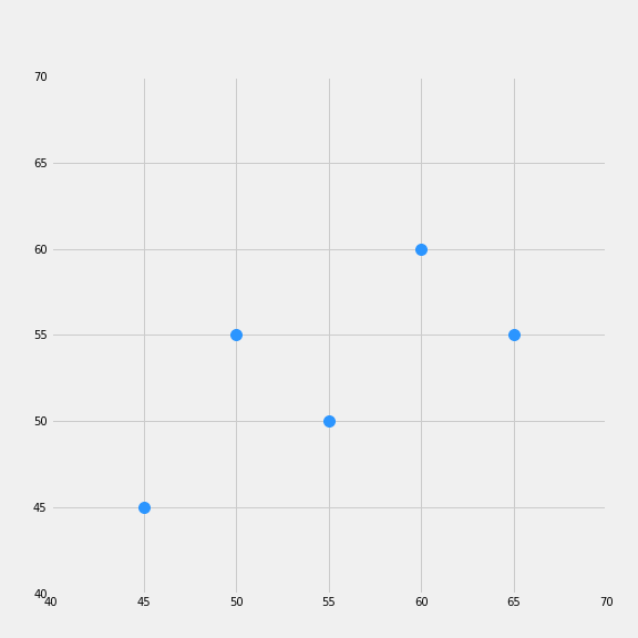
In the plot above, it appears that Y has an approximately linear relationship to X, meaning increases in x are typically accompanied by increases in y. It would, therefore, be of interest to find out to what extent this relationship can be described by a linear model. Let us assume our model takes the form:

Let’s plot an approximated best-fit line over our data.
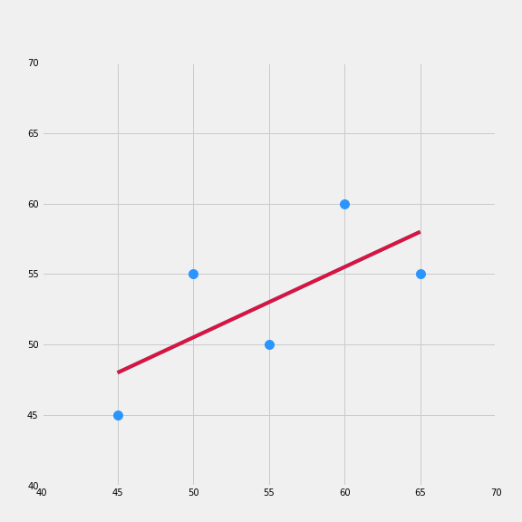
Our linear model fits the data pretty well, but it is not the best that we can do. In order to arrive at the best-fit line, we will need to use OLS, which entails approximating our slope coefficient and y-intercept by minimizing the sum of the squared distance between our data, yi, (the blue dots) and our model output yhat, the redline.
You might be thinking why do we need to square the distance? It turns out that because some points are above and below our estimates if we just try to minimize the sum of the distances, the values will offset. As long as there are points above and below the line, we will not arrive at a unique solution. Squaring the distances allows us to get around that by converting the values into absolute terms then we are allowed to minimize the sum.
The plot below illustrates this procedure.

Ordinary Least Squares Derivation
Mathematically, what we are trying to do is to minimize the squared differences:
1.)

From above we know that 
2.)
Inserting equation 2 into 1 we get:
3.)

In order to minimze equation 3 we will need use the chain rule and take the partial derivative with respect to both 


We can multiply both sides by -2 so we are just left with:
4.a)

4.b)

We can rewrite formula 4.a into the form:
5.a)

Remember the sum runs from 1 thru N so 

Since 1/N times 


we can multiply both sides by N and use them to cancel out the N in equation 5.a.
6.)


7.)

The last step will be to solve for 
8.)

Which we can rewrite as:

From equations 5.a and 5.b we can rewrite the equation as:

Next we can isolate beta and factor it out on the left side of the equation

Then we can solve for beta and we are left with

We know what alpha equals from the equation above

In the next section I will show you how we can solve for alpha and beta quite easily using Python.
Using Code to Solve for Our Parameters
import numpy as np
import matplotlib as mpl
from scipy import stats
import matplotlib.pyplot as plt
import matplotlib.style as style
%matplotlib inline
style.use('fivethirtyeight')
plt.rcParams["figure.figsize"] = [8,8]
mpl.rcParams["font.size"] = 18
mpl.rc('xtick', labelsize=10)
mpl.rc('ytick', labelsize=10)
#Using the formulas we derived above we can create our custom function to return alpha and beta
def regression(x,y):
xy = (x * y)
mean_x = x.mean()
mean_y = y.mean()
x_squared = sum(x**2)
beta = (xy - mean_x * mean_y).sum() / ((x - mean_x)**2).sum()
alpha = mean_y - beta * mean_x

return alpha, beta
fig, ax = plt.subplots()

xi =np.array([45.0, 50.0, 55.0, 60.0, 65.0])
y = np.array([45.0, 55.0, 50.0, 60.0, 55.0])
a, b = regression(xi, y)
# Generated linear fit
line = [a + b * i for i in xi]

plt.plot(xi,y,'o', color="#2b95ff", markersize=10)
plt.plot(xi, line, color="crimson")
#p = PatchCollection(patches)
plt.xticks([40,45,50,55,60,65,70])
plt.yticks([40,45,50,55,60,65, 70])
# for i in range(0,len(patches)):
#     ax.add_patch(patches[i])
plt.savefig('foo.png')
plt.figure(figsize=(3,4))
plt.show()
