Let’s face it, mean-variance optimization out of the box is all but useless. If you’ve ever used any kind of portfolio optimizer, you know that small changes to your initial inputs can often lead to concentrated allocations.

So as practitioners how can we get around this?

Add constraints to the optimization? Well, that sort of defeats the purpose. Reverse optimization? This assumes we know the weights of the global market portfolio(GMP). Risk Parity? What if we don’t have access to leverage?

Given that some of the issues in the optimization process are a result of small changes to our initial parameters, what if we simulate various capital market assumptions, optimize, and average across efficient frontiers?

This approach is called resampling and it can help us arrive at a more balanced allocation.

In this next section, I will walk you through an implementation of this process written in Python.

Every year J.P. Morgan publishes their long-term capital market assumptions. For the moment, let us assume these are accurate forecasts and use them as our initial inputs.

Fund	Expected Return	Volatility
U.S. Large Cap	6.4%	14.0%
U.S. Mid Cap	6.9%	16.0%
U.S. Small Cap	7.4%	18.8%
EAFE Equity	7.6%	17.3%
Emerging Markets Equity	10.0%	21.5%
U.S. Intermediate Treasuries	3.1%	3.8%
U.S. Inv. Grade Corporate Bonds	3.7%	6.0%
TIPS	2.9%	5.5%
U.S. High Yield Bonds	5.6%	8.5%
World ex-U.S. Government Bonds	2.6%	8.0%
Commodities	5.1%	16.8%

We will need to import a few libraries.

#import our libraries
import matplotlib.pyplot as plt
import pandas as pd
import numpy as np
from cvxpy import *
%matplotlib inline

Next, we need to:

• Use a multivariate distribution to simulate 10 years of monthly returns
• Calculate the expected return and covariances
• Optimize on those inputs and store the values in a Pandas Dataframe
• Repeat 500 times

 #create methods for optimization and simulation
def optimal_portfolio(returns):
n = len(returns.columns)
w = Variable(n)
mu = returns.mean()*12
Sigma = returns.cov()*12
gamma = Parameter(sign = 'positive')
ret = mu.values.T*w
risk = quad_form(w, Sigma.values)

prob = Problem(Maximize(ret - gamma*risk),
[sum_entries(w) == 1,
w >= 0.0])

SAMPLES = 100
risk_data = np.zeros(SAMPLES)
ret_data = np.zeros(SAMPLES)
gamma_vals = np.logspace(-2, 3, num=SAMPLES)
weights = []
for i in range(SAMPLES):
gamma.value = gamma_vals[i]
prob.solve()
risk_data[i] = sqrt(risk).value
ret_data[i] = ret.value
weights.append(np.squeeze(np.asarray(w.value)))

weight = pd.DataFrame(data = weights, columns = returns.columns)
return weight, ret_data, risk_data

def simulation(er, cov, sims):

#create date index
dates = pd.date_range(start='2018-08-31', periods = 120, freq='M')

data = []
# generate 10 years of monthly data using JPM estimates
for i in range(0,sims):
data.append(pd.DataFrame(columns = cov.columns,
index = dates,
data = np.random.multivariate_normal(er.values,
cov.values, 120)))
#store values from simulation
weights =[]
stdev = []
exp_ret = []
for i in range(0,sims):
#optimize over every simulation
w, r, std = optimal_portfolio(data[i])
weights.append(w)
stdev.append(std)
exp_ret.append(r)
return weights, stdev, exp_ret

With the above helper functions written, we will now need to import our data and run the code.

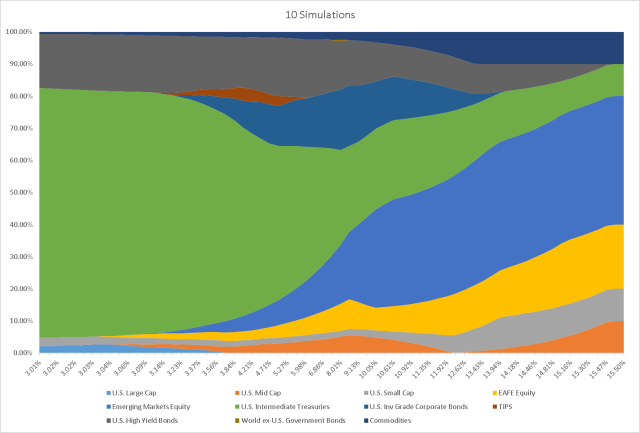
For now, let’s run 10 simulations in order to see how our allocations change as the amount of simulations increase.

er = pd.read_csv('er jpm 2018.csv', index_col = 0)['Expected Return']/12.0
cov = pd.read_csv('cov jpm 2018.csv', index_col = 0)/12.0
w1, stdev, exp_ret = simulation(er, cov, 10) # run 10 simulations

Plotting our data into an efficient frontier asset allocation area graph, what we see with only 10 simulations is an unstable/rigid allocation.

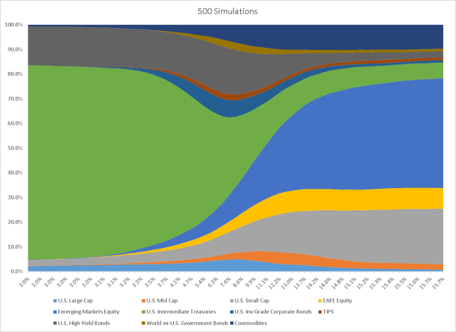
As we increase the simulations, in this case to 500, the plot begins to smooth out and we arrive at what appears to be a more stable/balanced allocation.

Conclusions:

In this post, we showed how it is possible to use Monte Carlo simulations in tandem with traditional mean-variance optimization to arrive at a more stable and diversified portfolio allocation. In order to improve upon this method, we may want to think about diversifying our capital market assumptions or including higher order moments into the optimization. While resampling is not a panacea for portfolio optimization, it is a useful tool to have in our tool chest.